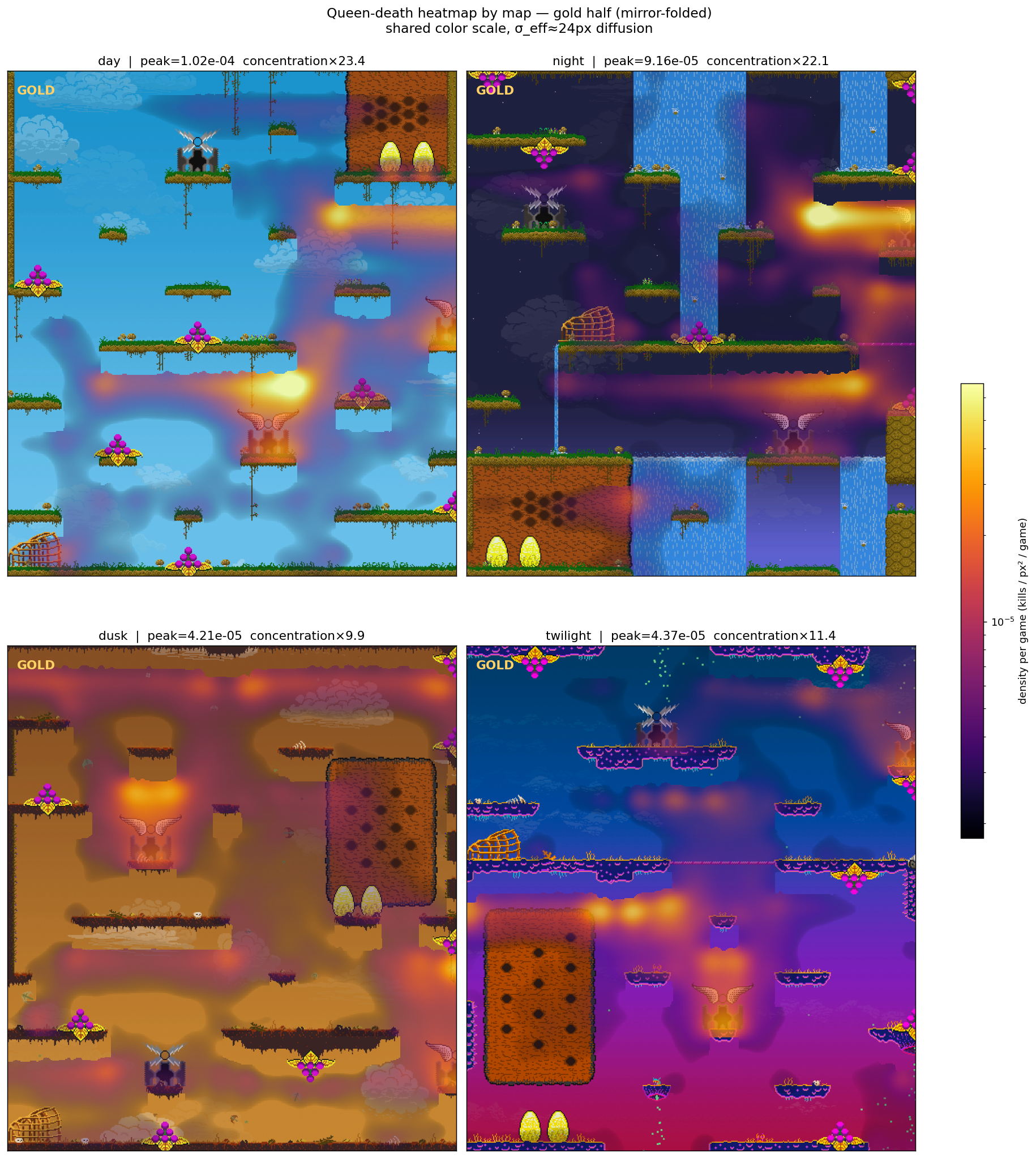
Inputs, transformations, and outputs. Each figure’s caption states only what was computed.
For each game in the quality-filtered set we walk the
playerKill events and keep
(killer_x, killer_y, killer_pid, killed_pid, killed_category)
plus the game’s map index, quality rank, and
gold_on_left flag. Positions are mirrored to a
canonical gold-on-left frame; y is flipped from Cartesian
(game) to pixel coordinates so it matches the screenshot.
Every quality-filtered game is included — 182,447 games in
total (49,147 day, 50,943 night, 47,427 dusk, 34,891 twilight),
6,096,016 kill events, 650,988 of them queen deaths. Where applicable,
both sides of a map are mirror-folded onto the gold half via
x' = min(x, 1920 - x), doubling effective sample density
in the visible area.
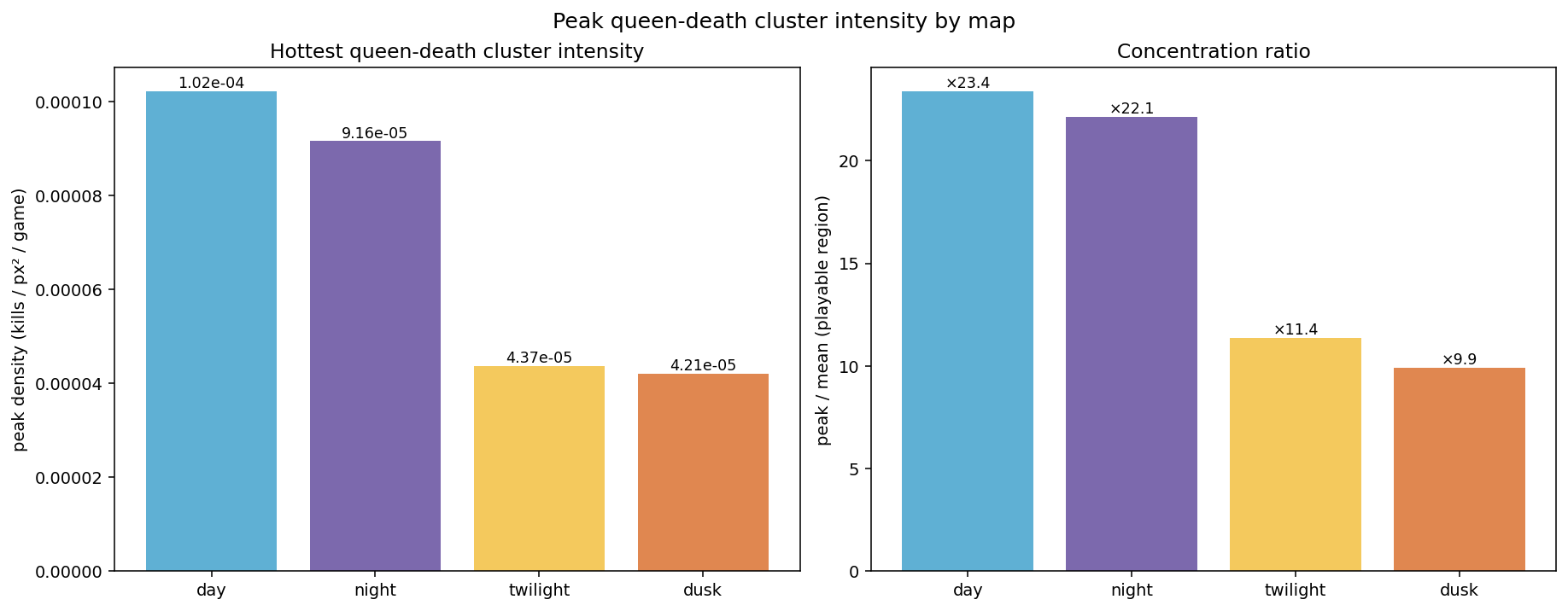
Wall-respecting diffusion (σ=24 px; algorithm in §4) run on each map independently with a per-map empirical mask. Densities are divided by the number of games sampled in that map so peaks are comparable across maps.
| map | games | queen deaths | deaths / game | peak density (kills/px²/game) |
concentration (peak ÷ playable mean) |
|---|---|---|---|---|---|
| day | 49,147 | 182,010 | 3.70 | 1.02e−4 | ×23.4 |
| night | 50,943 | 180,136 | 3.54 | 9.16e−5 | ×22.1 |
| twilight | 34,891 | 116,224 | 3.33 | 4.37e−5 | ×11.4 |
| dusk | 47,427 | 172,618 | 3.64 | 4.21e−5 | ×9.9 |
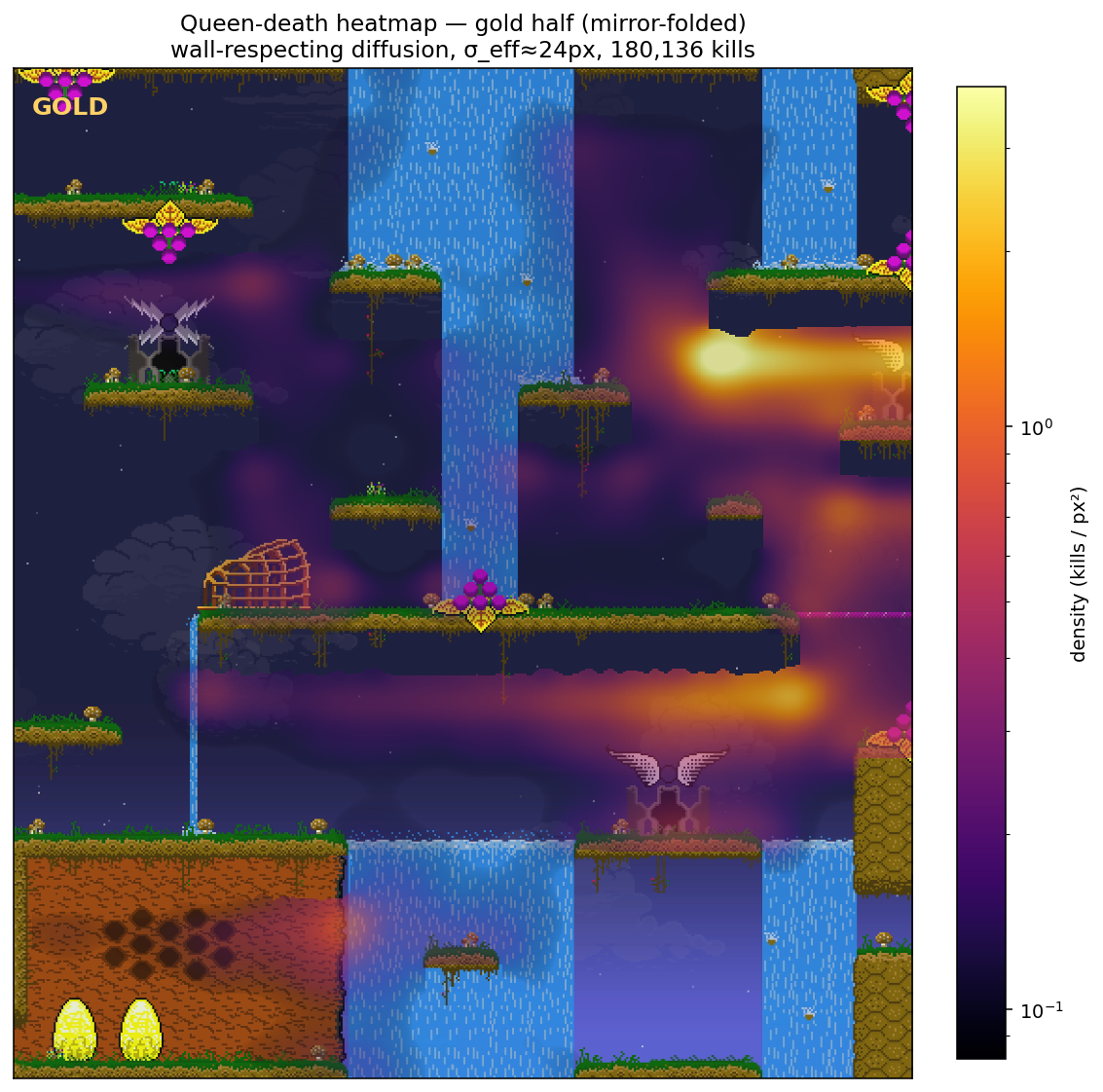
For each cell, two diffusion-smoothed densities:
D = density of queen-deaths (rows where
killed_cat == "Queen"; 180,136 events);
K = density of kills by queens
(rows where killer_pid ∈ {1, 2}; 701,574 events).
Plot log₁₀(D/K) minus the global value
log₁₀(ΣD / ΣK). Cells with low
combined signal (D+K below the 20th percentile of the
playable region) are masked out.
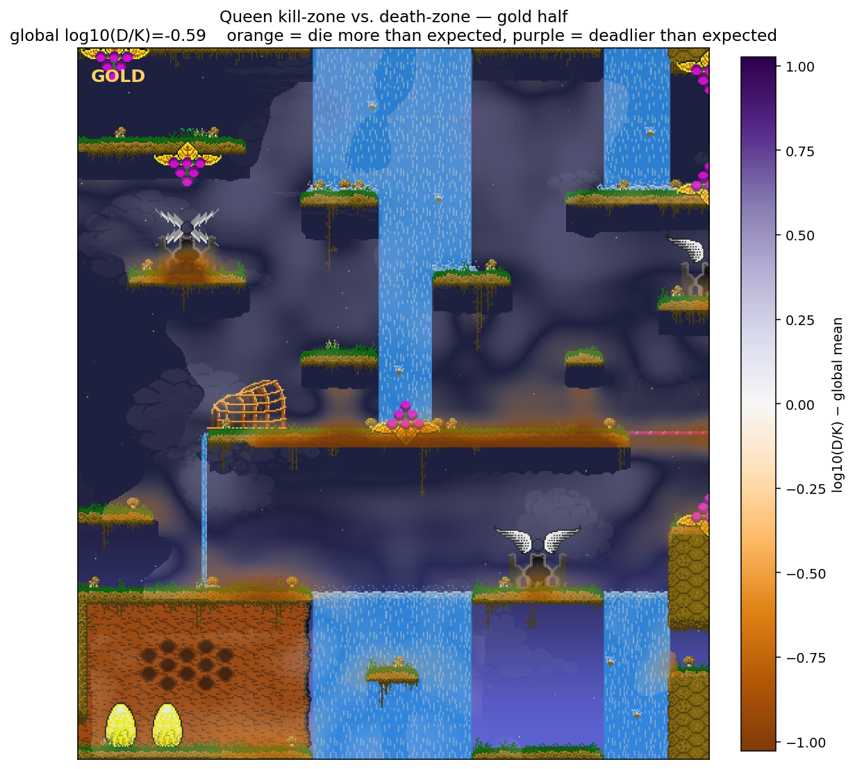
log₁₀(D/K) − global; alpha
proportional to |deviation| / vlim so cells matching the
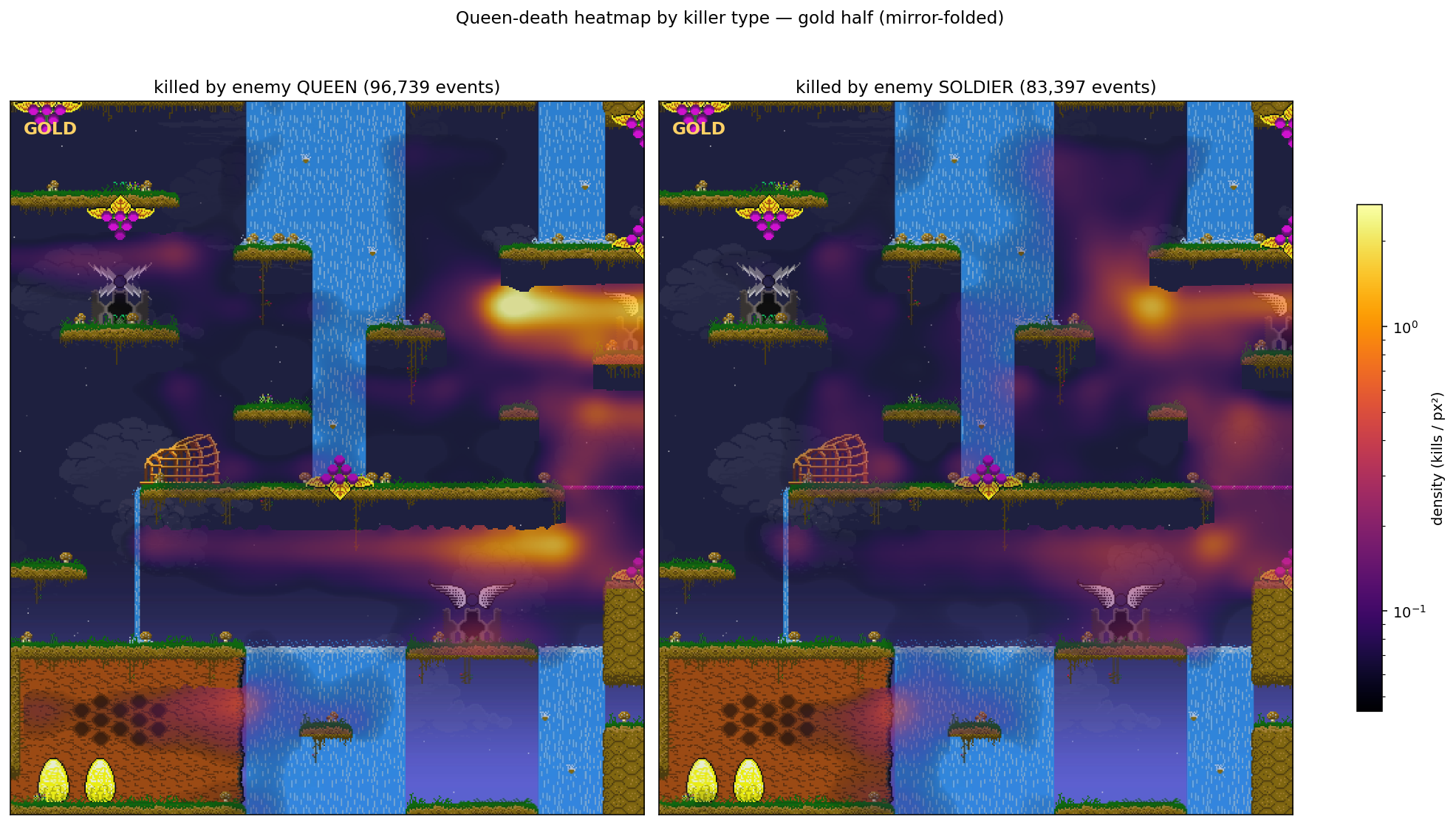
map average are transparent.Queen-death rows partitioned by killer:
killer_pid ∈ {1, 2} → killer is the enemy queen;
killer_pid ≥ 3 → killer is a worker, which must be
a winged soldier to have killed the queen. In the full night dataset,
53.7% are by enemy queen (96,739 events) and 46.3% by enemy soldier
(83,397 events).
The two densities recombined as a balance map:
log₁₀(Dₛₒₗₙᵢₑₐ / Dₑᴴᴴᴱₑₙ)
minus its global value
log₁₀(ΣDₛₒₗ / ΣDₑᴴᴴᴱₑₙ) = −0.06:
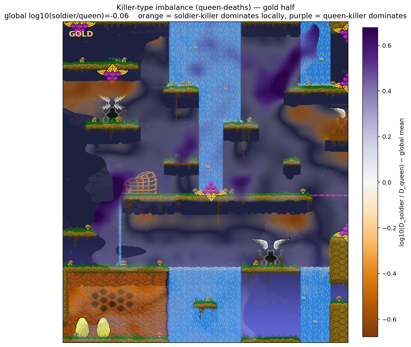
|deviation| / vlim.Kill positions are smoothed on a 2 px-per-cell grid using discrete Jacobi diffusion, with the playable region acting as a no-flux domain so density never crosses solid map geometry.
f ← H · M; mass on wall cells is zeroed.f(c) ← (1 - α) f(c) + α · meann ∈ N(c) ∩ M f(n)
with α=0.2 over the four orthogonal neighbours. Wall cells stay
at zero; their absence from the neighbour set is the no-flux
boundary condition.α·T cells²,
so we run T = round(σ2/α) iterations
to hit a target bandwidth. With cell size = 2 px
and target σ = 24 px, that’s
T = round(122/0.2) = 720 iterations.The result is rendered as an alpha-modulated overlay on the map
screenshot: alpha = 0.92 · progress^0.55 where
progress = norm(density) clipped to [0,1] and forced to
zero on cells with no density, so low-density cells let the map sprite
show through and high-density cells render opaque.